
This is a generic tool for manipulating a particle
Phase Space Density. It provides the capability to take a slice through
the distribution normal to an arbitrary vector as well as computing
the usual moments of particle distributions: density, bulk velocity,
pressure tensor, heat flux and temperature. It permits the user to
specify a spacecraft potential and an energy cut off for moments
calculation.
It is largely based on "Paschmann, G, AN Fazakerley, and SJ Schwartz: Moments of plasma velocity distributions, Analysis Methods for Multi-spacecraft Data, ISSI Scientific Report SR-001, 1998." Sets of parameters allow tuning the computation depending on the properties of the plasma and of the spacecraft.
It has been tested successfully by comparing its results to
those produced by the PEACE and CIS teams on some arbitrarily chosen
events.
You may contact the QSAS team at: csc-support-dl@imperial.ac.uk.
The input data set as a time series of arrays. The
data must be convertible to Joules ("SI_CONVERSION" attribute), and the
coordinates system must be spherical (either latitude or co-latitude for
the polar angle). The tool should be able to determine the axes
coordinates.
The "ENTITY" attribute is used to determine the mass and
charge of the particle, but these may also be manually selected.
There is an intrinsic ambiguity in the definition of Phase Space Density due to the possibility that the radial coordinate is given in terms of the flow direction or look direction. Note that CIS uses Flow direction, whilst PEACE uses Look direction. This tool sets the measurement direction parity automatically when either PEACE of CIS data are dropped into the PSD data slot, but at present this must be set manually for other data sets.
The Input PSD is usually in a local Spacecraft frame. On
Cluster, PEACE uses SR2 while CIS uses ISR2 (which is close to GSE). To
provide the output in a scientifically useful frame it is necessary to
provide the spacecraft spin axis latitude and longitude in either
GSE or GSM. The default is to assume GSE unless the Coordinate_System or Frame attribute is provided and set to GSM.
Alternatively, it is possible to provide a rotation matrix from the Data coordinate system to the target coordinate system.
The user can choose the output to be in either GSE or GSM (irrespective of the frame of Spacecraft axis Latitude and Longitude) or an arbitrary frame determined by the input rotation matrix.
It is possible to generate and save only the rotation matrix from Data frame to chosen output frame for later use in this tool or elsewhere.
This is used to compensate for the effect of the
particle acceleration in the vicinity of the spacecraft. The potential
is converted to energy by multiplying it with the particle's charge.
This
value is subtracted from the energies in the distribution. Any
resulting negative
energies are discarded.It may be supplied as a numerical value in volts,
or as a data object with a valid SI_conversion attribute. The default
is to assume volts.
The potential must be a non-negative value.
Energies under this threshold are discarded (applied before potential correction). This can be used to remove the effect of photoelectrons. No correction is done to compensate for the removal of this data. It may be provided as a numerical value in eV or as a data object with valid SI_conversion. The default is to assume eV.
The choice between sum over bins and integration over tetrahedra.
Summing over bins is much faster and when no corrections are applied
will produce results as accurate as integration over phase space
tetrahedra. Integration is likely to provide a better estimate when data
are missing or the distribution has been distrorted by potential or
energy cutoff corrections.
The moments of the PSD in the selected coordinate system
after taking account of the Spacecraft potential and selected lower
energy cut off. It is possible to select all provided moments or just a
selected subset using the tick boxes. The default is to generate only
the density.
This returns a two dimensional cartesian slice through the
PSD normal to a specified direction. Since it uses interpolation it is
possible to specify the number of bins required in (each dimension of)
the array. The result is in velocity space with axes binned in velocity
and the slice in units of per velocity cubed. The x and y axes in the
slice are equivalent to the x and y axes of the target frame when the z
axis is rotated into the direction of the selected normal vector.
Slices use the tetrahedral interpolation algorithm described below and can be slow to compute.
This returns a two dimensional cartesian slice through the
PSD normal to a specified direction. See above for the definition of
this normal and resulting X-Y axes of the slice. The velocity bins are
logarithmically spaced, with some extra added in closer to zero. A polar
version of this tool is planned.
Slices use the tetrahedral interpolation algorithm described below and can be slow to compute.
This returns a gyro-phase averaged pitch angle distribution
as a 2D array in polar coordinates, taking as inputs the velocity-space
origin from which to calculate pitch angles and the field direction.
User input includes the number of energy bins, pitch angle bins, and
also the number of gyrophase cuts, equally spaced in phi, used to
perform the average.
Pitch angle distribution calculations use the tetrahedral interpolation algorithm described below and can be slow to compute.
The rotation matrix from PSD frame to target frame is returned, but no other calculation performed.
Let E be an energy value. If E is lower than the photoelectron threshold, nothing is done. Else, E'=E+P.C, where P is the non-negative potential of the spacecraft and C the signed charge of the particle.
If E' is non-negative, it is converted into velocity v, knowing that 2E'=mv.v (m for the particle mass) and knowing the measuring probe coordinates (and the GSE transformation matrix).
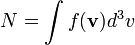
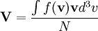
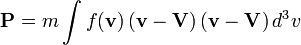
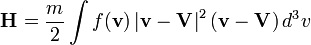
If f is the distribution function, the computed moments are:
This method is the faster of the two, it is also the most naive one. It simply consists in the sum of the elementary integrations over the bin volumes, simply approximated by multiplying the data values over the bin volumes.
In the following illustrations, the principles are shown on a
partial coverage of a 2D plane. The data values are shown as red
shades, and the bin boundaries are dashed lines.
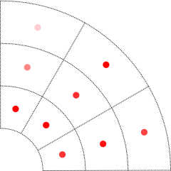
A part of the 2D plane is segmented into bins, each one carrying a value.
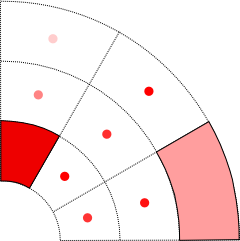
As illustrated on two bins, the integrated value is the value multiplied by the bin volume. These values are summed to give the total integrated result.
Despite its speed, this method is flawed when the data is sparse, as gaps are not filled.
In this method, the space is divided into tetrahedra
(triangles in the 2D illustration), which allow to fill the (convex hull
of the) space even if the actual data is sparse. Each vertex of a
tetraheadra carries a data value. These values are interpolated linearly
over each tetrahedra and then summed over all of these.
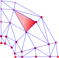
The space is covered by triangles, some points being added by the algorithm to better approximate the data space. As illustrated on one of these triangles, the values are locally linearly integrated.
The tetrahedrisation method used is a Delaunay tetrahedrisation implemented using a QuickHull algorithm.
Two successive iterations of this algorithm may give very slightly different results, as in an homogeneous distribution of points (as often in PSD) the Delaunay triangulation is not unique, and slight perturbations are introduced in the triangulation process to cope with numerical issues.