Profiles

Overview

QSAS can save user preferences as a configuration file, possibly holding multiple profiles. Parameters include for example default behaviour on dragging and dropping multidimensional data on the plot list, default plot page parameters, and default sizes for the main window and the plot interface window. These profiles are stored in user-dependent places: /Users/name/.qsasrc on Mac, /home/user/.qsasrc on Unix, and Documents and Settings/user/Application Data/qsas.ini on Windows.

The profiles are saved when QSAS is closed. Then QSAS opens with the configuration defined in the last-selected profile.

Editing and Using Profiles

The Profiles drop-down menu on the main window can select a profile to use or edit a profile.

Clicking Edit profiles... opens a Profiles Editor window, showing the setup for the currently-selected profile. Selecting another profile, using the pulldown at the top, displays the settings of that profile, discarding any unsaved edits made in the interface. The edits are made through various tabs, and can either be saved as a new profile (possibly updating an existing profile), or applied directly to a custom profile (which becomes the current profile) by clicking on Apply. The "Default" preset cannot be overwritten.

Items that only take effect after QSAS is re-opened are marked *.

Clicking a profile in the profiles list in the Profiles drop-down menu selects it as the current one.

Paths

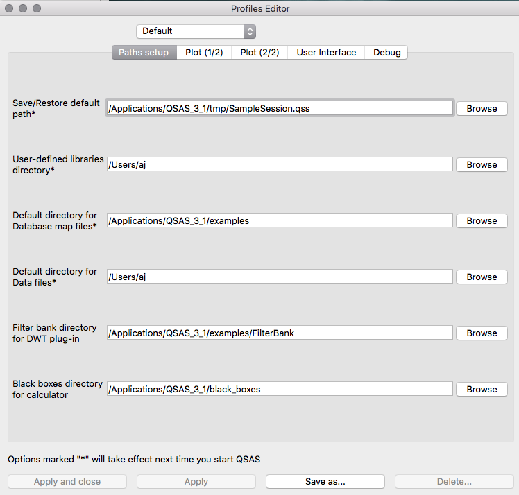
These options are accessible in the "Paths setup" tab. The first 4 paths are only taken into account when QSAS is opened, so they must be set up in the profile QSAS opens (last profile when QSAS was closed).

Save/Restore default path: the default path to save and restore sessions or the working list.
User-defined libraries directory: path for the qtpl and so/dylib/dll files for user-defined plugins.
Default directory for Database map files: for the Data Selector utility.
Default directory for data files: for open data file.
Filter Bank for DWT plug-in: for the Wavelet Transform plugin.
Black Box directory: for the calculator to add user saved black boxes.

Plot (1 of 2)

These options are in the "Plot (1/2)" tab.

Default behaviour when dropping a 3-vector: defines what is created by default when dropping a 3-vector in the plot list. Various combinations of panels are proposed.
Default behaviour when dropping a 3D array: either defines a summation on some components (iSS, SiS, iSS: the first, second and third components are untouched, respectively), or allows the user to explicitly define a summation/averaging rule. Presets are proposed.
Default behaviour when dropping a 3D array on a trace: either defines the summation (SSS) or the average of the components or allows the user to explicitly define a summation/averaging rule, to make a scalar series out of a 3D array series.
Default behaviour when dropping a 3D array as XY: defines over which components to sum or average, and the time element taken for a time series.
Time label format: defines the default set of separators for time labels.
Name of default Printer: needed for batch processing
Default page settings: defines the default parameters for the plot pages.

Plot (2 of 2)

These options are in the "Plot (2/2)" tab.

Fonts in plots: specifies the system fonts associated to the plot gui selectors. Check boxes for defaults. These are local parameters, not saved in the session. You can choose to vectorise fonts in svg exports, meaning that the fonts are drawn as vector objects, ensuring they are displayed correctly (but not easily editable).
Custom colour table: allow the users to specify their own colour tables, defined as interpolations of Hue/Saturation/Value (HSV) or Red/Green/Blue (RGB) values over a [0,1] range.
The format for HSV interpolation is HSV(0, H0, S0, V0)...(n, Hn, Sn, Vn)...(1, H1, S1, V1),
The format for RGB interpolation is RGB(0, R0, G0, B0)...(n, Rn, Gn, Bn)...(1, R1, G1, B1),
where
- the (n, X, Y, Z) 4-uplets associate the (X, Y, Z) colour to interpolation n (in [0,1]). Interpolation points must be in ascending order and defined at least for 0 and 1.
- R, G, B, S, and V parameters are defined in [0,1]
- H is defined in [0, 360] (red: 0, yellow: 60, green: 90, light blue: 180, purple: 270)
These are local parameters, not saved in the session. An example is given below.
Defaults for plot elements: Default values for some plot elements.

Custom colour table example

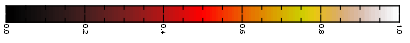
Let's define a colour table to represent heat levels for example, ranging from black for cold (low values) to red, yellow and finally white for maximum temperatures. We choose to define our colours in RGB representation. Their values are:

Black: all components at zero: (0, 0, 0)
Red: the red component is at its maximum value, the others are zero: (1, 0, 0)
Yellow: both red and green components are high, blue is zero: (0.8, 0.8, 0)
White: all components are maximums: (1, 1, 1)

We now have to choose the positions of these values on the scale. Black is at the bottom of the scale, hence 0, White is at the top of the scale, hence 1. We choose to put red in the middle of the scale, and yellow at 3/4. We finally obtain the following colour table description:
RGB(0,0,0,0)(0.5,1,0,0)(0.75,0.8,0.8,0)(1,1,1,1)

A similar colour table can be achieved in HSL mode, allowing more controls on the hues, and thus avoiding muddy colours that can appear interpolating over R, G and B components:

Black: (0, 0, 0) (red hue, no saturation, null intensity)
Red: (0, 1, 0.5) (red hue, full saturation, medium intensity)
Yellow: (60, 1, 0.5) (yellow hue, full saturation, medium intensity)
White: (60, 1, 1) (yellow hue, full saturation, full intensity)

The resulting syntax is: HSV(0,0,0,0)(.25,0,1,.5)(.75,60,1,.5)(1,60,1,1)

User interface

These options are in the "User interface" tab.

Default main window height: defines the main window height as a number of characters.
Default size for the plot interface: the plot interface window is too large for low-resolution screens, so it can be customised with this option. Resizing the plot interface and clicking "Get current size" gets the window size, which can be stored as a new default.
Font size in pixels: GUI font size, useful for smaller screens.
Show Toolbars at startup: if selected (default) the main window and plot window toolbars are shown on startup. The menu bar on the plot itself is unaffected and off by default.
Compact GUI: attempts to reduce the GUI size. For the moment, only reduces some margins.
WL slot pulldown: puts the pulldown arrow on data slots on right (default) or left.
Interactive interval editor button: button clicked to call the interval editor on a plot window.
Time Field Decimal places: controls the number of decimal places shown for seconds in time fields.
Start using Gregorian Calendar from: default date for use of Gregorian calendar. Only needed for really historical data! Different countries adopted it in different years.

Debug

The debug options allow extra feedback to the terminal when selected.

Tips/FAQ

Profiles make it quick to switch between two different behaviours, for example when dropping 3-vectors in the plot list interface. Create presets with the different behaviours you wish to apply.
The profiles files are ASCII and can be easily edited with any text editor. Syntax errors and unknown parameters are silently ignored. The profile files can be backed up and copied from any system to another (but the stored paths may be meaningless on some systems).

Last up-dated: October 2016 Tony Allen

Contents