Plotting
Polar and Cartesian 2D surface plots are available through a distinct window launched from the Plot menu on the QSAS main window as a separate Surface View menu item.
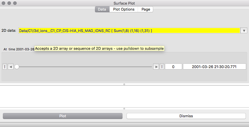
The Surface View window has three tabs, Data, Plot Options and Page and plots into its own plot window which is independent of the main plot window.
The Data tab has a data drop slot which expects a 2 dimensional array or array sequence. If a higher dimensional data object is dropped in it will use the default array reduction set in the user's profile in order to sub-sample down to 2 dimensions. This selection can be modified using the slot pulldown. When a time series object is dropped in, the record/time slider is active and the record to be plotted can be selected with the slider or typed into its record field. Changing the record will automatically re-plot the data at the new record.The Plot Options tab allows the user to control the plot design, but defaults for all options are set according to the data and its metadata. The plot and axis titles can be explicitly set in the appropriate fields. The Plot can be Mesh (mesh of surface triangles) and/or Surface Filled (solid blocks of colour for surface triangles) or Contours (contours at constant height offset from the base by their height value) or Histograms (Solid vertical bars for each bin bounded by the Delta_plus and Delta_minus values). The Axis Type field allows either Polar or Cartesian coordinates to be used, and when Auto detect is chosen (default) the axes will be polar if an angle variable is found as one of the dimensions. The Opacity of the surfaces can be set with Surface Opacity. Changing opacity can be viewed as changing the opacity at the bottom of the colour bar with a linear variation up to the top which is always opaque. Thus when Opacity is set to 1.0 all colours are opaque, and when it is set to 0.0 the top of the colour bar is opaque but opacity varies linearly to the bottom of the colour bar being transparent. Opacity may be negative, in which case the fully transparent colour is above the bottom of the colour bar.
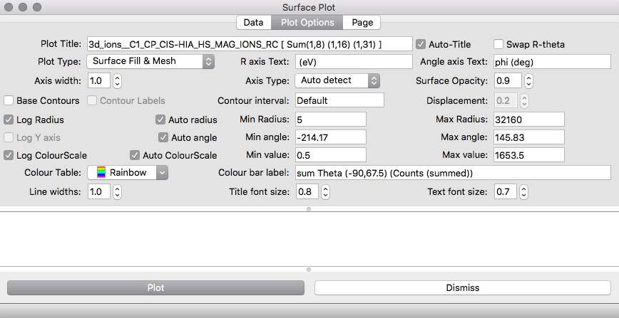
The Base Contours toggle will allow contours to also be plotted on the base plane, and all contour interval and contour labelling can be controlled. When a logarithmic colour scale is chosen the contour interval will refer to the interval in the power of 10.
The Radial dimension can be plotted in the log, in which case zero or negative radial values are automatically excluded. If the radial quantity is anywhere negative then, when log radius is selected, the minimum value in r is subtracted from each radial value and this offset noted in the text pane. In addition the first non-zero radial value is used as lower limit, but this may be over-ridden by manually setting the radial minimum value. Negative radial values are permitted for linear radial plots.
Similarly the data dimension (colourscale) may be logarithmic, in
which case the lowest non-zero value is used when autoscaling.
The colour scale range may be manually over-ridden.
The widths of lines used in axes, contours and mesh can be set using the
line width option, while title and label text can be controlled
independently.
The Page tab controls the paper size, resolution when printed (where appropriate) and paper orientation. Custom paper sizes can be specified, and all measurements are in the units set in the Units field. Page controls are the same as for the 2D polar plots.
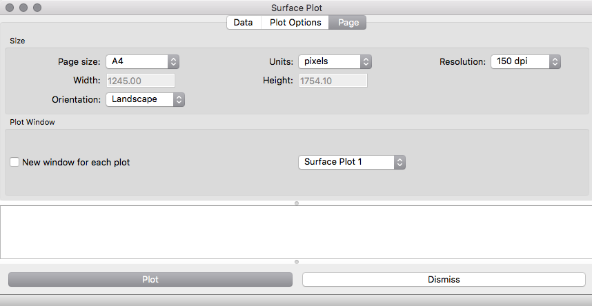
Under normal use each plot will appear in the same window created the first time Plot is pressed. The New window for each plot toggle allows a fresh window to be created each time Plot is pressed, and selecting the Plot window id of an existing window allows it to be overwritten (after deselecting New window for each plot).
The plot pane itself allows control of the viewing angle through sliders at the side and bottom. The viewing angle is then shown in the plot pane title bar.
The plot pane also holds an Animate View button which will continually change the viewing angle for 30 seconds, starting from the current viewing angle, and an Animate Time button which will successively plot each data record in the input data object from the current time slider position to the end. Animate Time will first calculate a suitable colourscale for the whole time interval if the Auto Colourscale toggle is on, and this may cause a delay before animation starts with large data sets.
Printing or saving a plot to a file is achieved using the Plot menu from the plot pane after plotting.
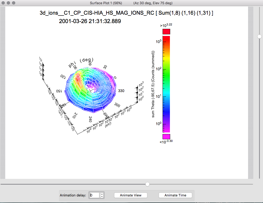
The Sample session shipped with QSAS contains a saveset
(saveSet.qx_surface_plot) for a 2D surface plot of the ion data in the
sample session.
The resulting plot should look as follows: