plotaz
Software to display and manipulate azimuthal slices of data from the
Cluster and Doublestar PEACE instruments (and perhaps other similar
instruments) from data held in the IDFS (see www.idfs.org) format.
plotaz draws on QPeace modules, which may have wider applicability. At
present, plotaz works correctly with the various 3-D PEACE modes,
including 3DX, 3DR, and LER, and also with PAD and SPINPAD data
(which are equivalent to the 3D products with only one sweep per "spin").
Contents
Copyright and License
Requirements
Authors
History
Running Plotaz
Using plotaz
IDFS Lineage
Energy/Velocity Options
Phase Space Options
Analysis Options
Plot Output
Save/Restore
Liouville Mapping and
Slicing
Concepts
Sources
Pitch Angles
Energy/Velocity
Units and Phase Space Units
Slices
Wheel Plots
Combined Wheel and
Slice Plots
Troubleshooting
Copyright and License
This software is made available under the GNU Public License. SwRI IDFS
software is licencsed separately and does NOT form part of this
software. Some of this software also uses freely available software
including the PGPLOT graphics library and the QT widget library. These
libraries are subject to their own licensing conditions.
Requirements
plotaz is distributed as a binary executable with dynamic linkage for
Linux (Mandrake) and Sun/Solaris. Various system and utility libraries
can also be found on the www distribution site if needed. The full
source code is delivered in the tarr'ed distribution.
plotaz is a C++ application, which draws on QPeace software, which
is written mainly in C. Separate programmer's documentation is provided
for generic QPeace routines. plotaz is a widget application using the QT
toolkit. It is developed primarily on a Linux workstation
(Mandrake) and tested regularly on Sun Solaris. Early versions were
developed on a Redhat system without difficulty. plotaz has also been
successfully built under MacOsX, and SwRI provides an SDDAS-aware
version which may be particularly helpful for MacOsX users and others
for whom the distributed binary code doesn't run properly and who do not
have access to the modules (especially idfs and perhaps pgplot) on which
plotaz depends. Graphics uses the C language interface to the PGPLOT
library (see http://www.astro.caltech.edu/~tjp/pgplot/).
In order to compile against IDFS modules, users will need appropriate
licensing authority for the IDFS software (see www.idfs.org).
Running plotaz requires a local pgplot xwindow server (pgxwin_server
- unless only gif and postscript file output is required) and a fully
functional SDDAS/IDFS system.
Authors
Steve Schwartz (s.schwartz@imperial.ac.uk) is the original author and
formal PEACE Co-Investigator.
History
26 November 2000 First issue; up-dated 20 June 2001
January 2002 Added attempt at autopromote (courtesy Joey Mukherjee,
SwRI); added capability to take a slice of a sweep, to map a sweep to a
new one based on specified potential difference, field magnitude, and
Liouville's theorem, and to plot all these results as line traces.
February 2003 Finalised autopromote; added function to add parallel
velocity shift in Liouville map to remove any parallel bulk velocity,
move into de Hoffmann-Teller or other special frame, etc.
February 2005 Up-dated to include gathering by multiple sweeps, spins,
or seconds, and correction for spacecraft potential. Also generally made
more robust against quirks in the data.
Running plotaz
Be sure the plotaz executable is in your search path (it is delivered
in the bin directory of the QPeace software), and that the pgplot
xwindow server pgxwin_server and fonts (grfonts.dat) are available,
e.g., by placing them in a directory and setting the environment
variable PGPLOT_DIR to point to that directory. plotaz should run
without these if the plots are sent to gif or postscript files. A script
PLOTAZ is provided which sets the shell and pgplot environment variables
if you do not want to add the PGPLOT_DIR environment variable to your
.cshrc. Edit this script to point to your local copies.
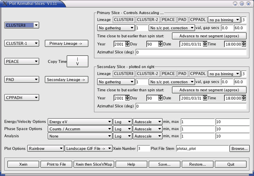
The application takes no arguments and brings up the single GUI
shown.
Using plotaz
IDFS "Lineage"
 Use the pull-down buttons on the left to
select the data source (virtual instrument) for the desired "primary"
azimuthal slices. Then push the "Primary Lineage ->" button to
transfer this information to the top right segment of the GUI. The
Primary Slice is used to autoscale the energy scale and counts/phase
space scales, and is also used to define the polar/energy bins for any
analysis. Type the time of interest in the Primary Slice time fields.
TIP: <Tab> takes you from one field to the next. The Advance to
Next Segment button will attempt to re-adjust the time to the next
equivalent segment (number of seconds, sweeps, or spins) depending on
the gathering and rebinning options chosen. This feature is not
guaranteed, and may skip some intervals, especially when used with PAD
data which has only two (SPINPAD has one) sweep per spin. Gathering by
sweeps (recall for SPINPAD 1sweep = 1 spin) is more reliable. For simple
sequences, the sister application qjas will plot a sequence of wheels in
addition to its special spectrogram plot, and such sequences are robust
in that the entire set is acquired and then cut into the relevant
pieces. This option is available under the plot file options.
Use the pull-down buttons on the left to
select the data source (virtual instrument) for the desired "primary"
azimuthal slices. Then push the "Primary Lineage ->" button to
transfer this information to the top right segment of the GUI. The
Primary Slice is used to autoscale the energy scale and counts/phase
space scales, and is also used to define the polar/energy bins for any
analysis. Type the time of interest in the Primary Slice time fields.
TIP: <Tab> takes you from one field to the next. The Advance to
Next Segment button will attempt to re-adjust the time to the next
equivalent segment (number of seconds, sweeps, or spins) depending on
the gathering and rebinning options chosen. This feature is not
guaranteed, and may skip some intervals, especially when used with PAD
data which has only two (SPINPAD has one) sweep per spin. Gathering by
sweeps (recall for SPINPAD 1sweep = 1 spin) is more reliable. For simple
sequences, the sister application qjas will plot a sequence of wheels in
addition to its special spectrogram plot, and such sequences are robust
in that the entire set is acquired and then cut into the relevant
pieces. This option is available under the plot file options.
Gathering
If you wish, you can gather any integral number of sweeps, spins,
or decimal time duration through the gathering pull-down menu above the
time fields.
Azimuthal Slicing (only if Gathering set to "No Gather")
Also select the azimuthal slice, in degrees from PEACE t_zero. Zero
degrees corresponds to sunward-flowing electrons, but as the spin axis
is directed approximately southward, the azimuth increases in the
opposite direction to, e.g., GSE azimuths (see the PEACE diagram for a guide to the PEACE
instrument, mounting, and coordinate systems). QPEACE software including
PLOTAZ converts directions as necessary to represent all velocities,
etc., as FLOW directions. The time corresponds NOT to the time of
the azimuthal slice, but to the beginning of the spin.
WARNING NOTE: Azimuthal slicing ONLY has meaning if the "No
gathering" option is chosen. In all other gathering options, the
gathered sweeps are all combined together and the resulting average is
plotted.
NOTE: The lineage buttons for Mission, Instrument, ... are NOT coupled
to one another to facilitate quick change from one spacecraft to
another, etc. This means that you can easily select a non-existent
combination, which will show up as a simple failure to open the selected
data source message on the console.
Secondary Slice
Similarly select the Secondary Slice parameters. If the lineage is
the same as the Primary, simply push the "Secondary Lineage ->"
button. The "Copy Time" button transfers the Primary Slice time to the
Secondary Slice box.
Pitch Angle Rebinning
Both slices offer the option of re-binning in pitch angle. This uses
high-resolution magnetic field data together with the instrument
measurements to calculate accurate pitch angles. The pull-down allows
the user to set equal size bins in either degrees or cosines (i.e.,
equal solid angles); the number of such bins is held in the right-most
boxes which are editable. All PAD (but not SPINPAD) and 3D data can be
rebinned this way if the field data can be found.
Spacecraft Potential Correction
Plotaz will correct the energy bins and, if appropriate, phase space
science values, for the effects of the spacecraft potential. This
correction can be given as a constant value in Volts, entered in the
first box to the right of the option pull-down, or extracted in the case
of Cluster from the EFW U_probe prime parameter data held in idfs
format. In the case of a gap in the EFW data larger than the value in
seconds given in the second text box, or if the EFW data is missing
altogether, the constant value is used. Velocities are converted to
energy, corrected for spacecraft potential, and then converted back
again.
The action taken in correcting the phase space science values
depends on the units selected (see Phase
Space Options below):
Phase Space Option
|
Action
|
Counts/Accumulation
|
None - preserve total counts
|
Phase Space Density (f(v))
|
None - Liouville's Theorem
dictates that f(v) is constant along particle trajectories, so assuming
that the spacecraft potential affects only the particle energy (and not
direction - the "scalar approximation") nothing needs to be done
|
Differential Energy Flux
|
Multiply pre-existing value by
(Enew/Eold)^2, corresponding to f(v) constant from old to new. The E's
are taken to be the mid-point of the energy/velocity bins.
|
PEACE and Plotaz Geometry
All angles are shown in FLOW directions; specifying an azimuth
of 0 degrees corresponds to particles travelling toward the sun (but the
spin axis is directed southward so PEACE azimuths increase in the
opposite sense to GSE. See the PEACE diagram).
A polar [or pitch] angle of 0 degrees corresponds to particles
travelling along the spin axis [or magnetic field in the case of pitch
angle distributions].
Energy/Velocity Options
Change these options as desired. Both energy (eV) and velocity (km/s)
are possible. Log scaling produces a double log axis. Note to specify
the energy min and max values on the plot you must change the pull-down
button to show "Userscale->" in addition to entering the values in
the corresponding boxes. After plotaz runs, the min, max boxes are
populated with the values used in the plots.
Phase
Space Options
Counts/Accummulation, Differential Energy Flux (essentially calibrated
and geometry-factor-applied counts) and phase space density are
provided. Options and scaling as per Energy/Velocity Options.
Analysis Options
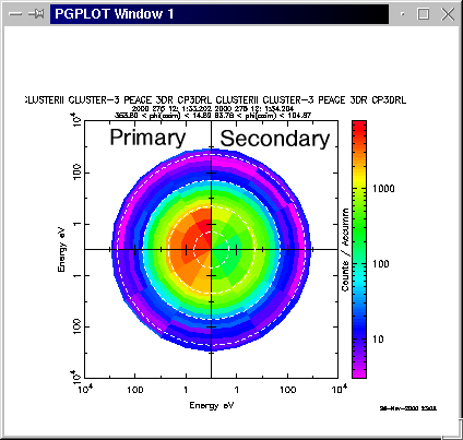
If none is selected here, pushing the Run button will result in a
single polar plot with the Primary and Secondary Slices on the left and
right respectively, as shown in the first example.
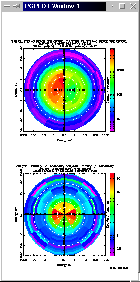 Selecting
any of the arithmetic options will result in two plots; the top shows
the individual slices, and the bottom the result of the indicated
arithmetic operation. If the two slices do not share the same
angle/energy bins, the second is interpolated onto the first prior to
the arithmetic operation. This interpolation is performed by converting
counts to counts/area and then mapping onto the Primary bins weighted by
the area of overlap between bins, before converting back to counts. In
the case of phase space density, this is mapped directly, weighted again
by area of overlap.
Selecting
any of the arithmetic options will result in two plots; the top shows
the individual slices, and the bottom the result of the indicated
arithmetic operation. If the two slices do not share the same
angle/energy bins, the second is interpolated onto the first prior to
the arithmetic operation. This interpolation is performed by converting
counts to counts/area and then mapping onto the Primary bins weighted by
the area of overlap between bins, before converting back to counts. In
the case of phase space density, this is mapped directly, weighted again
by area of overlap.
Plot Output
Several output formats are supported, including screen (X-window), gif,
and (encapsulated) postscript files in colour or grayscale. The Plot
File Stem box specifies the path and name of the desired output file;
.eps or .gif are appended as appropriate. [Pgplot eps files are not 100%
conformant in that they have the bounding box at the end of the file,
but most applications are happy with them. Google pgplot for more
documentation and environment variables.]
For X-window plotting, inserting an integer into the Xwin number box
will request pgplot to open and use that pgplot window. This enables the
user to retain more than one plot (by selecting different numbers on
successive runs) and/or to ensure that the application doesn't erase a
window drawn by another application. Pgplot X-windows are re-sizeable
and the output at the next Run is scaled accordingly.
Various environment variables can be set and are used by pgplot to
set plot page sizes. For example, here is an extract from a possible
.cshrc file (though these could also be put inside the plotaz_script if
desired):
setenv PGPLOT_DIR /usr/lib/pgplot
# A4 pages: ps defaults otherwise are 7800x10500 milli-inches
# Offsets from corner of page
setenv PGPLOT_PS_WIDTH 7560
setenv PGPLOT_PS_HEIGHT 10800
setenv PGPLOT_PS_HOFFSET 350
setenv PGPLOT_PS_VOFFSET 350
# GIFs: standard defaults are 850 x 680 pixels = 10 x 8 in [85 pix/in]
setenv PGPLOT_GIF_WIDTH 926
setenv PGPLOT_GIF_HEIGHT 638
# Xwindows default width as fraction of display width
setenv PGPLOT_XW_WIDTH 0.6
Save/Restore
As of version 3.10, plotaz can save to a single file all the entries
and selections on both the main gui and the subsidiary Slice'n'Map gui
to a file. The buttons bring up a file browser, and there are no
restrictions on file names or file extensions. The files are simple
ascii parameter-value files and can be hand-edited if desired. All
white-space is stripped, and all parameter names are in uppercase.
Selected items from pull-downs are stored by the order down the
pull-down menu, starting at 0. This method is not future-proof, and no
error-checking is performed, except that unrecognised parameter names
are ignored.
Liouville Mapping and
Slicing
Plotaz will also perform Liouville mapping of pitch angle distributions
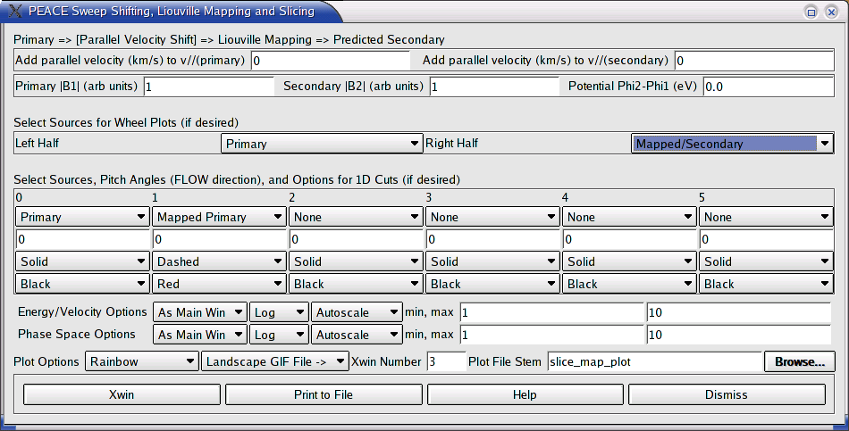
and can take slices of pitch angle distributions. Pushing the 'Run then
Slice'n'Map' Button on the Plotaz main gui will do two things:
- It will run plotaz as normal
- It will bring up the following secondary gui
Concepts
- Primary and Secondary refer to the azimuthal sweeps retrieved and
plotted in the main Plotaz gui
- Velocity shifting ADDS the speed inserted in the box to the
parallel component of all energy/velocity bins, and then interpolates
the result back onto a circular grid. The effect is essentially to move
the sweep in the 0 degree direction by this amount. The original sweep
is first increased in resolution to avoid leaving holes; the result is a
compromise between speed and quality (which could be altered by
recompiling after editing the entries in the plotaz header file). Both
primary and secondary sweeps can be shifted by independent amounts.
- Liouville Mapping (if desired) is performed on the PRIMARY sweep
by specifying the magnetic field magnitude corresponding to the primary
sweep and a new one at the "mapped" location - only the ratio of these
two fields is needed, so B1 can be left as 1. The electrostatic
potential difference between the "mapped" and primary location is also
needed. Liouville mapping assumes energy and magnetic moment are
conserved. See Chapter 7 by Schwartz, Daly, and Fazakerley, of Analysis
Methods for Multi-spacecraft Data (ISSI, Bern) for a thorough discussion
of Liouville mappint techniques and limitations. Mapping can be
performed on the original sweep, a parallel velocity shifted one, or
both.
- Pitch Angle Distributions are required for Liouville mapping,
although slices can be taken of any azimuthal sweep.
- Liouville Mapping can only be performed for sweeps
retrieved in PHASE SPACE DENSITY units, not counts, differential energy
fluxes, etc.
- "Pitch angles" for slicing and mapping assume the sweep is a
pitch angle one, with 0 degrees corresponding to the field-aligned flow
direction. Similarly positive and negative portions of the cuts
correspond to positive and negative FLOW directions respectively.
- "Pitch angles" are measured in the spacecraft frame; if the bulk
velocity is comparable to that of the electrons of interest, these pitch
angles and any mapping will not be appropriate unless the bulk shift is
applied.
- Gyrotropy/axial symmetry is assumed to obtain both positive and
negative portions of the 1-D slice. NOTE that for non-pitch angle data,
this algorithm does NOT give the slice along a single line; the + and -
halves are orientated differently.
Sources
One of
- None
- Primary - as retrieved in main Plotaz gui
- Shifted Primary - adding the parallel velocity specified in the
relevant box
- Mapped Primary - using Liouville's Theorem and summarised above
to generate a new pitch angle distribution based only on the original
primary sweep
- Shifted then Mapped Primary - using Liouville's Theorem to map
the primary sweep AFTER it has been shifted along the parallel axis.
- Secondary - as retrieved in main Plotaz gui
- Shifted Secondary
- Mapped/Secondary - the ratio of mapped to secondary, using the
arithmetic functions as described in the Analysis section for the main
plotaz gui
- Shifted Mapped/Shifted Secondary - ratio of the "Shifted then
Mapped" primary to the shifted secondary
- Mapped-Secondary - the difference of these two
- Shifted Mapped-Shifted Secondary - the difference of these two
Pitch Angles
are any real value in the range 0-180; values outside that range are
treated as 0 (if negative) or 180 (if > 180).
Energy/Velocity
Units and Phase Space Units
are those retrieved using the main plotaz gui, although the plot
scaling can be separately controlled in the Slice'n'Map gui.
Slices
For simple slices of sweep data, up to six traces may be selected using
the bottom half of the gui. If no wheel plots are requested, the plot
contains only slices as shown in the following example. Note that +0
degrees on the wheel plots corresponds to particles travelling along the
spin axis or, in the case of pitch angle distributions, +0 degree pitch
angle particles. The positive (toward the right) portion of the slice
corresponds to particles flowing in the direction of the chosen cut
angle. The negative portion corresponds to particles travelling in a
direction (180 - <cut angle>), so that both halves are taken from
a single (primary or secondary) source sweep wheel. Legends provide a
summary of the source, shifting, and mapping options together with
start/end time (for a quantity based on a single sweep) or start times
of the two sweeps in the case of arithmetic operations. Note/Caution:
the shifting (and to a lesser extent mapping) tends to exaggerate the
granularity of the original data.
Wheel Plots
These can be made from the same set of sources and specified using the
top portion of the Slice'n'Map gui. If no slices are specified, the plot
contains only the wheels, such as the following example which shows a
shifted then mapped distribution on the left and a distribution shifted
in the opposite direction on the right. [Note in this artificial example
the mapping yields a discontinuity at 90 degrees due to the large
velocity shift which created a large +/- asymmetry.]
Combined Wheel and
Slice Plots
These are generated by selecting sources in both the Wheel and Slice
sections of the gui, and produce a single page.
Troubleshooting
Launching
Most problems launching plotaz are related to either library
inconsistencies between the supplied binary versions and the user's
local installation. Try downloading the collection of system libraries
from the qpeace homepage, put those in the qpeace/lib directory, and
uncomment/edit the PLOTAZ script to put these libraries ahead of your
own system's in the LD_LIBRARY_PATH environment variable. Other things
such as the pgplot shareable (.so) library may also need to be added to
your LD_LIBRARY_PATH in the same way. If the application fails saying it
can't find a xyz.so file, that's what the problem is, so make sure you
can find the file it's looking for and put it in the LD_LIBRARY_PATH.
Lineage
Most problems stem from:
- the specification of the IDFS lineage being incorrect, or
- no data being held locally for the requested time
Note that the elements making up the lineage are treated independently,
so it is possible to specify a non-existent lineage. On the other hand,
this makes selecting the same virtual instrument on another spacecraft
quite easy and quick.
plotaz silently does nothing in these circumstances, though some
error messages may be written to the console from which it was launched
which may be helpful
Plotting
If the plot fails to appear on the screen, this is probably a problem
with the pgplot installation. Pgplot may issue an error message to the
console.
- check to ensure that there is an environment variable PGPLOT_DIR
set which contains the pgxwin_server and grfonts.dat file.
- try generating a gif or postscript file
- check if pgplot re-used a plot window which is displayed on a
different "desktop"
If a plot file is specified but doesn't appear, perhaps plotaz was
launched from a directory other than the one in which you are looking
for the file. Try specifying a full path for the file.
Bugs and Features
plotaz tries to identify missing values prior to any arithmetic,
although in practice the default missing value is taken to be zero..
Thus in the division of one slice by another, a value of zero
corresponds to one of zero, infinity, or a missing value in one of the
original slices.
plotaz SHOULD now (as of version 3.0) handle PAD data in HAR mode. It
should handle the SPINPAD equivalent (which can NOT be re-binned in
pitch angle using high resolution magnetic field data).
Advancing to the next segment is prone to errors which may result in
skipping an extra spin. This is due to some interaction between idfs
file opening/positioning and subsequent fetching. For PAD data,
selecting gather by 1 sweep (SPINPAD <=> no pitch angle binning)
is more reliable as it avoids trying to find the start of a spin.
Pitch-angle rebinned PAD seems less prone to this problem.
Report bugs and comments to: s.schwartz@imperial.ac.uk
Peace Diagram
Page maintained by: Steve Schwartz (s.schwartz@imperial.ac.uk)
Last updated: 9 May 2007