qjas
Software to display angle-time spectrograms stacked by energy of
data from individual energy sweeps of the Cluster and Doublestar PEACE
instruments (and perhaps other similar instruments) from data held in
the IDFS (see www.idfs.org) format. The plot format is based on a design
developed by J-A Sauvaud, CESR, Toulouse. When viewed from afar, the
separate spectrograms merge to resemble an omni-directional energy-time
spectrogram. Within each spectrogram, the angular dependence of a given
energy level is revealed.
qjas will also export such sweep-organised data to an ISTP/Cluster
compliant CDF file or to a flat ascii file with attached header
conformant with the Cluster Exchange Format adopted for the Cluster
Active Archive (see DS-QMW-TN-0010.pdf).
qjas draws on QPeace modules, which may have wider applicability. At
present, qjas works correctly with the various 3-D PEACE modes,
including 3DX, 3DR, and LER, in which the angle dimension corresponds to
polar angle of each sensor; as time advances successive sweeps are
plotted together with a panel showing the asimuth. Qjas also renders the
original PAD data and the newer SPINPAD (which is equivalent to the 3D
products with only one sweep per "spin") in which the angle dimension
corresponds to pitch angle. As of Version 3.0, QJAS will gather a
user-specified number of sweeps, spins, or seconds with options to rebin
in energy, to correct for spacecraft potential using the Cluster EFW
prime parameter probe potential or a constant value, and to rebin onto a
user-specified pitch angle distribution using high-resolution
magnetometer data.
Contents
Copyright and Licence
Requirements
Authors
History
Running qjas
Using qjas
IDFS Lineage
Energy/Velocity Options
Phase Space Options
Plot Output
Wheel Sequences
Data Export
Save/Restore
Troubleshooting
FAQ
Copyright and License
This software is made available under the GNU Public License, with
copyright by the author(s). SwRI IDFS software is licencsed separately
and does NOT form part of this software. Some of this software also uses
freely available software including the PGPLOT graphics library and the
QT widget library. These libraries are subject to their own licensing
conditions.
Requirements
qjas is distributed as a binary executable with dynamic linkage for
Linux (Mandrake) and Sun/Solaris. Various system and utility libraries
can also be found on the www distribution site if needed. The full
source code is delivered in the tarr'ed distribution.
qjas is a C++ application, which draws on QPeace software, which is
written mainly in C. Separate programmer's documentation is provided for
generic QPeace routines. Qjas is a widget application using the QT
toolkit. It is developed primarily on a Linux workstation
(Mandrake) and tested regularly on Sun Solaris. Early versions were
developed on a Redhat system without difficulty, and it has also been
built successfully on a MacOsX platform. A build is supplied by SwRi as
an SDDAS-aware application, which is probably particularly helpful for
Macintosh users. Graphics uses the C language interface to the PGPLOT
library (see http://www.astro.caltech.edu/~tjp/pgplot/).
In order to compile against IDFS modules, users will need appropriate
licensing authority for the IDFS software (see www.idfs.org).
Running qjas requires a local pgplot xwindow server (pgxwin_server -
unless only gif and postscript file output is required) and a fully
functional SDDAS/IDFS system.
Authors
Steve Schwartz (s.schwartz@imperial.ac.uk) is the original author and
formal PEACE Co-Investigator.
History
20 June 2001 First issue
31 July 2001 Includes file export
January 2002 File export conforms to Cluster Exchange Format; attempt
to include data promotion (courtesy Joey Mukherjee, SwRI).
July 2002 Added rebinning in pitch angle and custom energy bins.
February 2005 Significant re-write of qpeace idfs routines to perform
better with data quirks, sun pulse, jitters, and other afflictions of
real data. Added capability to gather (i.e., average) variable numbers
of sweeps, spins, or seconds, and to correct energy limits (with
corresponding corrections to science values if appropriate - e.g.,
differential energy flux), for spacecraft potential.
Running qjas
Be sure the qjas executable is in your search path (it is delivered in
the bin directory of the QPeace software), and that the pgplot xwindow
server pgxwin_server and fonts (grfonts.dat) are available, e.g., by
placing them in a directory and setting the environment variable
PGPLOT_DIR to point to that directory. qjas should run without
these if the plots are sent to gif or postscript files. A script QJAS is
provided which sets the shell and pgplot environment variables if you do
not want to add the PGPLOT_DIR environment variable to your .cshrc. Edit
this script to point to your local copies.
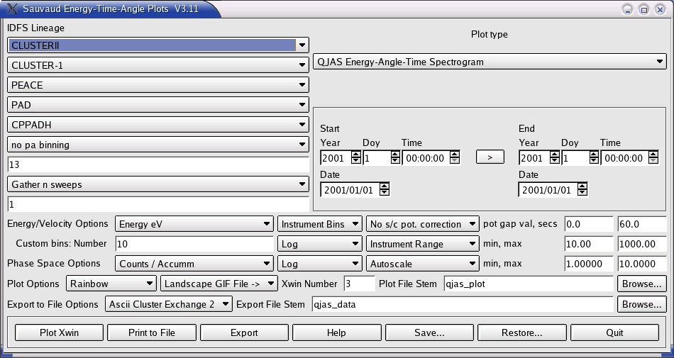
The application takes no arguments and brings up the single GUI
shown. Pushing the Help button brings up a text browser containing this
documentation.
Using qjas
- IDFS "Lineage"
- Use the pull-down buttons on the left to select the data source (virtual instrument) for the plot. Here you can also choose to re-bin the data into pitch angles (in the spacecraft reference frame) using high resolution magnetic field data (for PAD, LER, and 3D data). The edit box allows you to specify the number of bins, which can be equally spaced in angle or cosine from the pa binning options pull down. Also here you can specify whether to gather the data by an integral number of sweeps or spins, or by a decimial number of seconds. This operation effetively averages over the corresponding sweeps. By default, qjas gathers one sweep at a time. All scaling options on counts preserve the total number of counts and so distort the resulting distribution; use differential energy flux for physically meaningful normalisation. Pitch angle rebinning and multiple sweep gathering can be done simultaneously. [Pitch angle rebinning gathering one spin from version 3.0 of QJAS is roughly equivalent to the pitch angle rebinning performed by versions 2.x. However, the results are not identical, as the order in which these operations are done has changed, and the data are first pitch angle binned on a grid of their original resolution. Although this implentation was done for technical reasons, it also produces a better result, with fewer holes and in keeping with the inherent resolution of the data.]
Type the times of interest in the time fields.
TIP: <Tab> takes you from one field to the next.
The "Copy Time" button transfers all entries in the start time to the end time, after which you can edit the appropriate end time field, e.g., to plot one hour of data.
- Energy/Velocity Options
- Change these options as desired. Both energy (eV) and velocity (km/s) are possible. Instrument bins uses the bins as gathered by the instrument. Custom bins allow you to choose the number, scaling, and range of bins. Interpolation is performed based on a pseudo-spherical polar algorithm. You may also correct the energy bin limits for spacecraft potential. The "Do s/c pot. correction" option will attempt to open the EFW prime parameter files as held in idfs, extract the probe potential, and estimate the spacecraft potential as 1 - probe potential. If a gap larger in seconds than the (editable) number in the final text box on this row is detected, including when there is no EFW data at all, the value shown in the penultimate box (defaulted in the image above to 0.0 Volts) is used instead. If the "Constant s/c pot" option is chosen, the value shown in the box is used to correct all the data. The correction is performed by subtracting the spacecraft potential (interpolated down to the time of the sweep) from the energy bin limits (or by correcting the velocity appropriately). For phase space quantities of counts, no adjustment is made (so that the result preserves total counts). For phase space density, no adjustment is made due to an appliation of Liouville's theorem, which preserves f(v) along particle trajectories (assumed here to be unaltered in direction but changed in energy). For differential energy flux, the science values are adjusted by the square of the ratio of new to old energy at the midpoint of the bin.
- Phase Space Options
- Counts/Accummulation, Differential Energy Flux (essentially calibrated and geometry-factor-applied counts) and phase space density are provided. Options and scaling can be adjusted using the pull-down menus and editing the appropriate fields. On return, the actual values used in the plot are shown in the min/max boxes. Note that to specify min/max values the pull-down selection must show "Userscale" or the entered values will be ignored and the plot autoscaled.
- Plot Output
- Pushing the run button will generate a plot covering the requested time interval, as shown in the example below.
- Each horizontal band is an angle-time spectrogram for a single energy band. The centre energy (or velocity) is shown down the left side of the plot.
- Within each band are "Instrument FLOW Angles". The angle scale is shown to the right of the top-most energy sub-panel. For 3D data, this angle is the polar FLOW direction corresponding to each the anode. For the original PAD data and SPINPAD, this angle is the FLOW angle of a measurement with respect to the magnetic field direction, so that fluxes ascribed to 0 degree FLOW directions correspond to particles travelling in the same direction as the magnetic field vector (0 degree pitch angles).
- The bottom-most panel shows the PEACE azimuth corresponding to the measurement. Zero azimuth corresponds to a plane containing particles FLOWing toward the Sun, based on the spacecraft configuration and PEACE reset 3.8 degrees after the Sun pulse. For PAD data this is the angle through which LEEA rotates from start of spin to be looking in +B direction. This azimuth may be in error and should not be trusted. Note that since the spin axis points southward, the PEACE azimuth increases in the opposite direction to the GSE azimuth. See the PEACE diagram at the end of these notes.
- Several output formats are supported, including screen (X-window), gif, and (encapsulated) postscript files in colour or grayscale. The Plot File Stem box specifies the path and stem name of the desired output file. The suffix ".gif" or ".eps" are added to the stem name. [Pgplot eps files are not 100% conformant in that they have the bounding box at the end of the file, but most applications are happy with them. Google pgplot for more documentation and environment variables.]
- For X-window plotting, inserting an integer into this box will request pgplot to open and use that pgplot window. This enables the user to retain more than one plot (by selecting different numbers on successive runs) and/or to ensure that the application doesn't erase a window drawn by another application. Pgplot X-windows are re-sizeable and the output at the next Run is scaled accordingly.
- Various environment variables can be set and are used by pgplot to set plot page sizes. For example, here is an extract from a possible .cshrc file (though these could also be put inside the QJAS script if desired):
- setenv PGPLOT_DIR /usr/lib/pgplot
# A4 pages: ps defaults otherwise are 7800x10500 milli-inches
# Offsets from corner of page
setenv PGPLOT_PS_WIDTH 7560
setenv PGPLOT_PS_HEIGHT 10800
setenv PGPLOT_PS_HOFFSET 350
setenv PGPLOT_PS_VOFFSET 350
# GIFs: standard defaults are 850 x 680 pixels = 10 x 8 in [85 pix/in]
setenv PGPLOT_GIF_WIDTH 926
setenv PGPLOT_GIF_HEIGHT 638
# Xwindows default width as fraction of display width
setenv PGPLOT_XW_WIDTH 0.6
- Wheel Sequences
- As of version 3.10 qjas will generate a sequence of wheel plots (like those output by the sister application plotaz) to either the designated X-window or to a set of sequentially named gif files. This option is found under the Plot Type pull-down on the top right of the application window. Each wheel is a symmetric (left=right) representation of the same information contained in one verticle strip of the qjas spectrogram, and has been gatherered and binned in exactly the same way. Autoscaled ranges are based on the first strip, so you might want to fix the colour scale range to that in the qjas format (which autoscales over all sweeps; this is easily accomplished by first plotting a qjas plot, then changing the Phase Space options from Autoscale to Userscale to fix the values.To step through the X-window sequence, you need to hit return in the console from which the application was launched. In the QPEACE bin directory you will find scripts to rename the wheel sequence files by pre-padding the numbers with zero to make the alphabetic order agree with the numeric order (e.g., changing plot2.gif to plot00002.gif so that it precedes plot00010.gif) and also a version of that script which will also turn the multiple gif files into a single animated gif using gifsicle (http://www.lcdf.org/~eddietwo/gifsicle/). Gifsicle is an easy to install and use gif manipulator and viewer.
- Data Export
- qjas will also export the same data it uses in its plot, namely multiple 2-D angle-energy sweeps. Output includes all energy-angle bin information (written for each record to cope with changing instrument modes). Three output formats are supported:
- Ascii Cluster Exchange format is a flat comma-delimited data file with an attached header. The file format conforms with the Cluster Exchange Format (cef2) adopted by the Cluster Active Archive, although the earlier exchange format is still available. For readability, each variable is put on a separate line; 2-D arrays, in particular the sweep data, is broken into rows corresponding to the rows of the matrix. [cef specifies C-ordering for arrays, with which the above is consistent for 2-D arrays]
- Ascii Tabular (qft) is similar to the above but the data entries are in tabulated fields for easier reading. Note that for large arrays, line lengths become very long and not all editors/systems handle these particularly well.
- CDF files roughly conforming to ISTP/Cluster standards.
- The Export File Stem box is used to hold the path and output file name stem; the suffices ".cef", ".qft", or ".cdf" are added as appropriate to the file name.
- Save/Restore
- As of version 3.10, qjas can save to a single file all the entries and selections on the qjas gui. The buttons bring up a file browser, and there are no restrictions on file names or file extensions. The files are simple ascii parameter-value files and can be hand-edited if desired. All white-space is stripped, and all parameter names are in uppercase. Selected items from pull-downs are stored by the order down the pull-down menu, starting at 0. This method is not future-proof, and no error-checking is performed, except that unrecognised parameter names are ignored.
Troubleshooting
Launching
Although not especially verbose, qjas does issue various warnings and
errors to the console window from which it was launched, and this may
provide clues as to the source of the problem(s). Most problems
launching qjas are related to either library inconsistencies between the
supplied binary versions and the user's local installation. Try
downloading the collection of system libraries from the qpeace homepage,
put those in the qpeace/lib directory, and uncomment/edit the QJAS
script to put these libraries ahead of your own system's in the
LD_LIBRARY_PATH environment variable. Other things such as the pgplot
shareable (.so) library may also need to be added to your
LD_LIBRARY_PATH in the same way. If the application fails saying it
can't find a xyz.so file, that's what the problem is, so make sure you
can find the file it's looking for and put it in the LD_LIBRARY_PATH.
Lineage
- Most problems stem from:
- the specification of the IDFS lineage being incorrect, or
- no data being held locally for the requested time
- Note that the elements making up the lineage are treated independently,
so it is possible to specify a non-existent lineage. On the other hand,
this makes selecting the same virtual instrument on another spacecraft
quite easy and quick.
- qjas silently does nothing in these circumstances, though some
error messages may be written to the console from which it was launched
which may be helpful
Plotting
- If the plot fails to appear on the screen, this is probably a
problem with the pgplot installation. Pgplot may issue an error message
to the console.
- check to ensure that there is an environment variable PGPLOT_DIR
set which contains the pgxwin_server and grfonts.dat file.
- try generating a gif or postscript file
- check if pgplot re-used a plot window which is displayed on a
different "desktop"
- If a plot file is specified but doesn't appear, perhaps qjas was
launched from a directory other than the one in which you are looking
for the file. Try specifying a full path for the file.
Exporting
- First make sure the lineage and time are valid, e.g., by plotting
the data.
- Most cdf problems are due to an error or missing CDF_BIN or
GENERIC_PATH not being set correctly. CDF_BIN should point to the system
directory containing the executable skeletoncdf. GENERIC_PATH should be
set to point to the directory which contains a copy of the skeleton file
generic.skt [this is supplied in the distribution in QPEACE_HOME/bin].
- Other general problems are usually due to write permission
errors. Try setting a full pathname and file in the file stem box, e.g.,
- /home/sjs/output_file which you are certain you have write
permission for.
Bugs and Features
- qjas tends to use a value of zero as a missing or indeterminant
value (e.g., divide by zero), although it attempts to use the missing
value supplied in the original idfs data file.
- pgplot will truncate filenames (which can include paths as well)
after 80 characters. For wheel sequences, qjas appends "#.gif" to your
file name, where # is the position of the sequence number. If this is
beyond 80 characters, the 2nd and subsequent names default to
"pgplot#.gif" and end up in your current working directory.
Report bugs and comments to: csc_support@qmul.ac.uk
FAQ
Q: Why don't I always see the full set
of energies when I know the instrument returned more?
Q: When I correct for the (varying) spacecraft
potential, why do my plot and exported data not show varying energy bins?
Q: When I correct for the spacecraft
potential, the colours and values in the plot change. Why?
Q: How are count rates treated in
rebinning or correcting for spacecraft potential?
Q: Why does gathering sweeps of PAD
data result in twice as many output time strips when rebinned in pitch
angle?
-------------------------------
Q: Why don't I always see the full set of energies when I know the
instrument returned more?
A: To plot (and export), QJAS always recasts the data onto a
uniform set of energy/angle bins. The template for this interpolation is
taken by default from the FIRST sweep being plotted/exported. You can
change this by selecting Custom Bins, and then specifying a new number
and energy range for these bins.
Q: When I correct for the
(varying) spacecraft potential, why do my plot and exported data not
show varying energy bins?
A: The QJAS code does indeed use the instantaneous value for the
spacecraft potential, and each sweep of data is corrected accordingly.
However, before plotting or exporting the data, they are interpolated
onto a COMMON set of energy/angle bins, taken to be those of the FIRST
sweep in the sequence. The interpolation algorithm finds the overlapping
polar area between the old and new bins and computes a weighted average
of the phase space density within each new bin.
Q: When I correct for the spacecraft
potential, the colours and values in the plot change. Why?
A: Correcting for spacecraft potential involves converting to
(presumed) free space values for phase space density. In essence this
means following electron trajectories from the spacecraft back in time
and applying Liouville's Theorem. This theorem tells us that proper
phase space density f(v) is
conserved in this process, and you should see that when you are looking
at phase space density the colours do not (interpolation matters aside)
change. However, differential energy flux (DeF) is proportional to E^2 f(v), and qpeace software thus
calculates a new DeF by finding the ratio of E^2(new) to E^2(old) in
order to preserve the associated value of f(v).
Q: How are count rates treated in
rebinning or correcting for spacecraft potential?
A: All qpeace operations on count rates are designed to preserve the
total number of counts. This can be misleading if you try to interpret,
say, pitch angle rebinned count rates in terms of the underlying
distribution function. At the same time, it is a useful measure of where
the instrument counting statistics really are (and aren't). If you want
to do physics, use a physical quantity. Differential energy flux is
essentially the same moment of f(v) as the instrument count rate, so you
can think of DeF as calibrated counts.
Q: Why does gathering sweeps of PAD
data result in twice as many output time strips when rebinned in pitch
angle?
A: When NOT rebinned, PAD actually fetches and uses the SPINPAD
virtual instrument (you can see this in the title to the plot). SPINPAD
has two separate measurements, a half spin apart from one another,
combined into a unified pitch angle distribution. Gathering by sweeps
grabs each individual piece of this and rebins it in pitch angle
separately, resulting in twice as many results. This is useful if you
want to see where/when the various contributions to the pitch angle
distribution were sampled (and indeed the time resolution corresponds to
the precise instrument sweep). To get the analog to the SPINPAD
data, pa-rebin the PAD data by gathering SPINS instead. You may
also specify two sweeps, though in some instrument modes (HAR) there are
more than just two sweeps returned, so gathering by SPINS is more robust
(unless you want to see those extra sweeps).
PEACE Diagram
Page maintained by: Steve Schwartz (s.schwartz@imperial.ac.uk)
Last updated: 9 May 2007 (AJA)