
QSAS: A Science Analysis System for Space Plasma Data
Analysis
QSAS enables the user to perform various kinds of analysis and manipulation of data. In all cases, the operations are performed on objects held on the Working List, and the results of the analysis are, in general, returned as new objects on the Working List from which they may be further manipulated, plotted, or exported.
The main types of manipulations in QSAS are:
The Calculator provides a graphical interface for assembling and saving chains of analysis operations. All Analysis operations are available to the calculator.
Launches the Phase Space Density tool. It can to slice data normal to a vector, or create moments of the distribution or generate a pitch angle distribution given the magnetic field. See the PSD documentation.
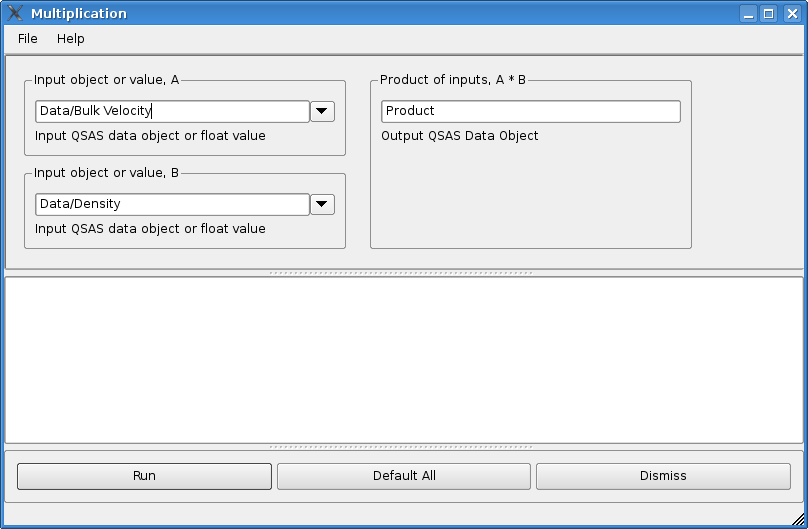
The Analysis/Simple Maths menu on the Main Window of QSAS provides direct access to a number of arithmetic operations. These open a window with slots for the input data objects and names of the output object(s) as shown. The Help button provides some detailed information. A new window is opened each time an arithmetic option is selected from the menu so multiple operations can be repeated with different inputs. The arithmetic input slots accept any type of numeric data input.
Input Arguments can be objects from the Working List or integer, floating point or text constants typed directly in the input slot. Constant vectors can also be created using the New Object option in the Edit menu on QSAS Main Window. Binary operations on time series data will automatically join the second object onto the timetags of the first. Binary operations involving a data/time series and a constant value will apply that constant value to each element of the data/time series.
Output objects are created and placed on the Working List with the name(s) given in the slot(s). These output objects include Units (text strings) and SI_conversion (formatted information) appropriate to the operation. Thus, in the example shown, the object Product will have Units = "km/s /cm^3" (straightforward concatenation of the two Units attributes) and an SI_conversion = "1.e+9>m^-2 s^-1" meaning multiply the values by 1.e9 to convert them into the SI standard units. Other operations, such as addition, are checked for compatible SI_conversions and warnings given if they do not appear to be appropriate.
QSAS chooses the applicable operation for the input arguments. Thus the same interface is used to multiply a vector time series by a numeric constant (input as 2.0 , or just 2), or multiply two scalar time series, as in the example, or multiply a vector by a rotation matrix (either a single matrix or a series of matrices on the same time tags). It is safe to experiment with arithmetic operations as conformality of input objects is checked at run time and a warning issued if the result cannot be varified (such as metadata being unavailable) or the operation is rejected if the result is invalid or ambiguous (such as adding two objects with different SI_conversion values).
QSAS can convert an object's units in any sensible unit using the SI_conversion attribute of the object. The Analysis/Change Units menu offers three ways of changing the units of an object:
Analysis of time-ordered datasets often requires data to be placed onto
a common set of time tags prior to further analysis. For example, taking
the difference between two time series of plasma density, e.g. n1(ti) and
n2(tj) requires that each time ti at which n1 has a value has a matching
tj so that n1(ti) - n2(ti) can be found. Since often n1 and n2 come from
different sources, this is not usually the case, and one or both of the
series n1 and n2 must be interpolated, averaged or otherwise manipulated
so that new series n1* and n2* can be differenced. This matter is critical
and complex, and the interested reader may wish to consult Chapter 2 (Time
Series Resampling Methods by Harvey and Schwartz) in the ISSI book Analysis
Methods for Multi-spacecraft Data published by ESA/ISSI and available in
electronic form at the ISSI web-site. Generally, when the target timetags
are widely spaced with respect to the original set, simple boxcar averaging
(with a boxcar twice as wide as the target timetag spacing) is appropriate.
For closely-spaced target timetags, linear interpolation is often as good
as more sophisticated techniques. In all cases, gaps in the time series
need to be trapped and either filled or entries removed.
Note that QSAS will make these choices appropriately when joining is
done on the fly, and for many operations joining first is not necessary.
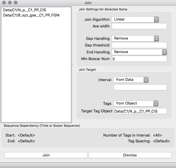
The QSAS Join routine, accessible from the Analysis/Time Ops.. menu on the Main Window of QSAS, enables the user to control all aspects of joining time series. All objects to be joined are placed into the list on the left. These need not be all the same type, e.g., they could be a mixture of scalar, vector, and array time series. The source of the target timetags is specified in the lower right portion. This can be one of the input objects, but could be another time series (i.e., any data object which has a set of corresponding timetags), and an option to create a set of regular time tags with specified spacing is also provided (which are needed if Fourier methods are to be employed).
The resulting objects will all be given the same suffix ending to their names on the Working List.
The upper right panel enables the user to select the interpolation/averaging options and gap treatment, and to specify corresponding parameters. The options chosen apply to the highlighted object(s) on the join object list, and different options may be set for different input objects or groups of objects.
Like the Working List, it is possible to group objects into folders on the join list for convenience if many objects are to be joined at once.
Note that selecting the Fill Value option for filling gaps may result in data series of different lengths if the 'Strip Fill Values' toggle is set on in the QSAS main window. Objects joined with this gap handling choice may therefore fail future tests on whether the data are joined, even after they have been joined.
Similar behaviour will result if a zero fill is selected for gap handling if the fill value (held in the Fillval attribute for the object) is also set to zero.
Data objects from different sources may need to be "synchronised" to reflect the propagation of a physical phenomenon for example. The Time Shift and Time Stretch options in the Analysis/Time Ops... menu allow these changes. The first one takes as an input a time series objects and am offset in seconds, and produces an object on the working list that corresponds to the input object with shifted time tags. The second option takes 3 inputs: the time series whose time tags need to be shifted and stretched, a reference time interval, which can be the object's time interval itself, and a new interval, onto which the reference interval is mapped.
The Time Series Subset option works as a filter, removing
from an input object the data not fitting in a specified time interval,
and outputting the result as a new object on the Working List.
Make Monotonic will remove any records out of time order.
Various operations are possible converting between timetags and seconds from a time value.
These operations remove records from a series based on different conditions.
These operations are specific to three vectors.
These operations are specific to arrays.
These operations support simple statistics.
Sequences of events are called Event Tables. These can be manipulated as follows:
These apply to data that are angles, or are being treated as such, and similar operators.
This provides an interface into the sub-sample and sub-dimension
tools available in data slots, with the option to save as a new object.
The three point method will tolerate unevenly spaced data, and will
use a two point estimate for the first and last data point and start
and end points of any data gap.
The Interface allows the user to set the data interval to be treated as
a data gap, but this will default to 1.5 times the spacing of the first
two data points in the series.
The five point method will create evenly spaced data using the
spacing of the first two data points and will linearly join across any
gaps.For situations where the data are not
regularly (or very nearly regularly) spaced the five point estimate
will not give better accuracy than the basic three point method.
The definite integral is evaluated over the whole selected data range
and returns to a single number (or single vector or matrix), while
the indefinite integral is the cumulative integral at each record and is
hence equivalent to the indefinite integral with unknown constant of
integration. Both definite and indefinite integrals may be performed in three ways.
Access to user-written plug-in routines is provided through the Browse option in Plug-Ins pull-down menu on the Main Window of QSAS. A file selection window enables the user to locate the template (*.qtpl) file corresponding to the desired plug-in. The QSAS supplied standard plug-ins are accessible directly through the Analysis and Geophysics sub-menus of the Plug-Ins menu. Currently supplied plug-ins include a suite of magnetospheric coordinate transformations, minimum variance and spectral analysis routines, time-lagged cross-correlations, and a cluster locator.
Use of a plug-in is identical to the use of Arithmetic described above (indeed, all the Arithmetic routines are actually written as plug-ins, and provide useful examples for users wishing to write their own plug-ins).
The QSAS Plug-in interface allows user-written routines to be compiled independently from QSAS. Writing Plug-ins is described in separate QSAS documentation. Briefly, a plug-in consists of a C++ wrapper routine, which accepts the input arguments from the Working List and returns the Output objects to the Working List. This wrapper in turn passes the inputs to the user's routine and collects the results. The user's routine may draw on the C++ methods of the DVOS objects to perform many tasks directly on the input objects (such as addition, masking, joining...) or may unpack the object to pass simple arrays to routines written in C, Fortran, or some other language. Indeed, since control is passed from QSAS to the plug-in, a plug-in may in turn display its own graphical user interface, do its own plotting, or launch an independent package. Finally, an ASCII template file tells QSAS information about the input and output arguments, from which the initial Graphical User Interface is constructed and presented to the user.
Other Plug-ins will be added, and users are encouraged to submit their own routines for wider distribution (or requests for other plug-ins they would like to have!). The Refresh Menu item in the Plug-ins menu will reread the Analysis and Geophysics directories to update the list of Plug-ins available through the pull down menus, and this allows newly added plug-ins to become immediately available to an already running QSAS session without restart. Similarly, if a .qtpl template file has been removed from the Analysis or Geophysics directories the corresponding menu item will be removed by the Refresh Menu action.
As plug-ins are loaded dynamically and given program control, some care is required to ensure that plug-ins are robust against improper inputs. If a plug-in crashes, it crashes the rest of QSAS with it.
Page created by Steve Schwartz, csc-support-dl@imperial.ac.uk
Last up-dated: October 2016 Tony Allen