QSAS: A Science Analysis System for Space Plasma Data

Introduction

Contents:

• Overview
• User Interface
• Mouse Behaviour
• Data Objects and Time
• Object Drop Slots
• Toolbars
  
• Getting Started
• Restore Sample Session
• Data Ingestion
• Export
• Saving
• Quitting
• Tips/FAQ

Overview

QSAS is a multi-platform application for the analysis and display of time series data. Specifically it is tailored for data from space plasma missions. It can ingest, manipulate, display, and export science data, and pays particular attention to the associated "metadata" (units, reference frames, etc.). Most space plasma measurements are made sequentially in time, and QSAS has been specifically designed with this in mind.

QSAS is based around three concepts:

• Data Handling

  Data ingestion is achieved either via an advanced hierarchical view of data held in a database or by simply opening a file. Once ingested, data together with metadata (reference frame, units, etc.) are held in internal data objects and available to the user from the Working List on the main QSAS window. Data objects are referenced by text names.

  Data objects may also be exported to files in either Common Data Format (CDF) or as ASCII flat files.

• Data Analysis

  Data objects may be manipulated by in-built analysis routines, such as arithmetic or time series joining algorithms and a built in calculator with graphical interface. Additionally, user-written plug-ins may be utilised through a dynamically-built interface allowing specialised routines to be created and made available without re-building the entire QSAS executable. Many plug-ins are distributed with QSAS. The results of all analysis routines are returned to the Working List for use in further analysis or display functions.

• Display

  A flexible panel plot interface allows the user to construct panel plots drawing data from any object on the Working List. Interactive cursor use enables the user to expand plots and/or save time intervals which may be passed to other analysis routines or control the plotting ranges of other panels.Specific 2D and 3D visualisation tools are also provided.
  

User Interface

QSAS is an interactive application, and the interface conforms largely to standard graphical user interface (GUI) conventions such as the use of pull-down menus, buttons, selectable scrolling lists, pull-down option menu buttons, and such. A few key concepts and actions are worthy of note here.

Mouse Behaviour

• Selection (highlighting of a Working List Data Object) is performed by a single click of the left mouse button
• Information/Action is sometimes performed by a double click. For example, double click on objects held in the working list on the main QSAS window will result in a browse and edit window on the object contents and properties.
  
• Drag and Drop is used extensively throughout QSAS. This is accomplished by a "down" left button over the desired object (which doesn't actually need to be selected first), dragging it keeping the button depressed until it is over a drop site and then releasing the mouse button. This works also on groups of objects selected with multiple selection. QSAS will bring the underlying window to the top when any visible part of it is under the mouse during drag, so to access a drop site not immediately visible, first drag across another part of the target window, then back to the newly revealed drop site.
  
• Multiple Selection A selection may be extended within any of the lists of QSAS objects. Holding down the shift key while making further selections will select all objects between the original and final selections, while control clicking will add (delete if already selected) from the selection. Only object lists accept drop from a multiple selection. Drag on a multiple selection is initiated with a single left "down" exactly as for single selections.
• Copy and Paste can usually be used as an alternative to Drag and Drop. Depending on the keyboard and window manager (and window) Copy can be accomplished by one or more of: Copy key, Ctrl+C, right click and select copy, with matching Paste functions performed by Paste key, Ctrl+V, right click and select paste. Most fields also accept the typing of text directly by the user. The last drag operation is normally stored in the copy register and the drop operation may be repeated using paste.
• Right Mouse Button brings up a context sensitive menu of operations that may be performed on the selected object, such as move, copy, delete etc. On the Mac this is control-click.
  
• Interactive Graphics Cursor selection is done by dragging a rectangle using the left mouse button.

Data Objects and Time

• Data Objects form the underpinning of all QSAS functionality. They include ingested variables, the results of analysis routines, time intervals, and constants. Internally, QSAS data objects are C++ objects which include metadata (descriptions, names, cross-references to other objects or timetags, units, etc.). For efficiency, all data objects are held in active memory.
• Management of data objects is accomplished from the scrolling lists on the Main QSAS window using either right click and selecting an option from the pop up menu, Ctrl+up/down arrow to move (and other shortcuts), drag and drop and double click to pop up a browse and edit window. Management includes ordering the lists for convenience, creating subfolders and deleting objects to free up memory.
• Names of data objects (and the path if they are in folders) are used to pass the objects from one window to another, by "drag and drop", "copy/paste" or direct text entry. Names are resolved to the underlying object only when some analysis/action is instigated, but each object on a list of objects knows the full path and name of the object it refers to on the Working List. Therefore, replacing an object on the main window "Working List" with another of the same name will result in the second object being accessed by all other GUIs which have that object in a Drop slot. This behaviour minimises confusion and enables previously used analysis or display configurations to be re-used on similar data, e.g., from another time period.
• Time Interval objects can be created and edited in many ways, and hold a pair of ordered Start-Stop times. QSAS stores time as Universal Time without leap seconds.
• Event Table objects are edited as sequences of Time Intervals. They can be converted from/to VO table files.
  

Object Drop Slots

In windows where data objects are to be used there will be appropriate drop slots to receive the dragged object. They also accept a typed name with path or typed numeric or text value. These slots also give the user the option to subsample on dimension or time via a pulldown menu.

See QSAS Array Reduction.

Toolbars

Getting Started

QSAS is run from a script which ensures that the appropriate local paths and environment variables are set. User-specific parameters are stored in profile files, which can also be edited easily manually (~/.qsasrc on Unix and OSX, Documents and Settings\User\qsas.ini on Windows).They can also be edited using the profiles menu on the QSAS main window.

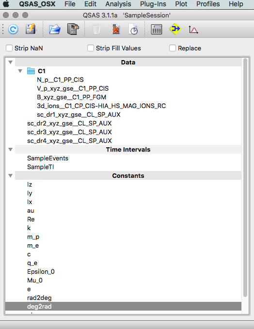
On launching the QSAS (or QSAS.bat) script the QSAS Main Window, containing a Working List of Data Objects, will appear. This is the centre of all QSAS operations.

Restore Sample Session

As a very brief introduction, pull-down the File Menu and select Restore Session. The resulting File Selection widget should be navigated to the /tmp directory of the QSAS installation. Select the SampleSession.qss directory and click OK. This will restore a session with some Cluster Summary Parameter data, and particle counts arrays, placing the data objects on the QSAS Working List.

Double click one of the Data objects on the Working List to browse the data and metadata attributes. The same Data Browser is used throughout QSAS. This Browser also allows you to edit both the data and metadata associated with the object.

Pull down the Plot menu and open up the Plot Layout. You will see the layout which was saved in the Sample Session. Pushing the Plot button will give you an on-screen plot. The plot Window can be resized, but the aspect ratio of the plot is constant to reflect the page format.

Note that the spectrogram at the bottom was plotted from the 3D ion distribution (for a different time period with its own T-axis) using the pulldown menu on the input data slot. For this plot the array was summed over both angle dimensions to give a 1D array time sequence for a spectrogram binned in energy. The same array reduction pulldown could have sliced the data at a specified bin or taken a subset by selecting only certain bins for inclusion.

You can modify many aspects of the Plot. Try multiple-selection of the the first three Traces by clicking on Data/B1_xyz_gse__C1_PP_FGM [x], then Ctrl-Click on Data/B1_xyz_gse__C1_PP_FGM [y] and Ctrl-Click again on Data/B1_xyz_gse__C1_PP_FGM [z]. The Right-hand side of the Plot GUI now shows you options for the selected items, some of which will be grey to indicate either that the selected items have different entries in that field. Select the Trace Tab and choose a new colour for the traces by pushing the Colour button, then Plot.

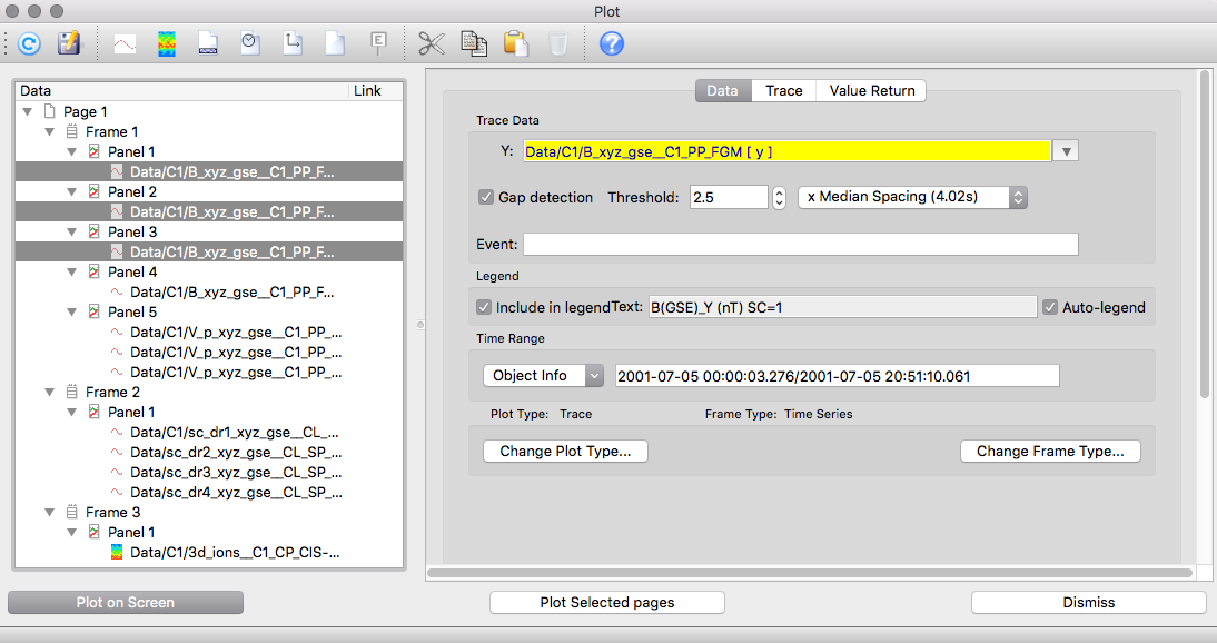
Frame 1 shows the use of the plot legend, which is normally used for multiple traces in a single plot, while frames 2 and 3 show use of rotated axis labels.

Now select Frame 3 in the list on the left, which will select everything underneath it in the hierarchy. The Tabs on the right provide control over various aspects of the Time Series Frame (a vertical collection of panels which share a common time axis). Select the T Axis tab. Now, from the Working List on the QSAS Main Window, Drag the "SampleTI" Time Interval onto the White Drop Slot called "From Object". Pushing Plot will then restrict the spectrum plot to the time interval specified by "SampleTI". By double clicking "SampleTI" on the Working List, you can edit the time interval to which it refers, and then push plot to investigate other time intervals. You can also change the plot time interval, and/or the time interval associated with a Time Interval object on the Working List, interactively. To do so, select the Value Return tab. Pushing the "Get Values" button will launch the Interactive Value Return GUI. Select a time interval by dragging a selection rectangle within a panel. Return to the Value Return GUI, uncheck "Rescale Y axis" and press "RePlot" to check your time range. Pushing "Save X T interval" will save this to the Working List with a specified name. Drop that new object into a T Axis drop slot (or several) to interactively select various time intervals of interest. Such Time Intervals can also later be used by Analysis routines.

Selecting Frame 3 again, T axis tab, and selecting "Autoscale" from the "Use" combobox box will return you to the full time range.

Now Delete the entire Page. Multiply select several objects on the Working List and drop them onto the blank hierarchy. QSAS will create a separate frame or for each which depending on where they are dropped. The Panels can be moved to occupy the same frame, and the empty frames then deleted. If first you create a new Frame and then drop objects onto it, QSAS will put the new panels onto the same Frame.

QSAS can perform simple analysis. There are three principle routes for performing analysis, individual operations under the Analysis menu, the Calculator and externally written plugins.

The Calculator menu on the "Analysis" menu launches a unified join and calculate window. The sample Session shows this being used perfrm a simple de-trending. The calculator can chain operations together, with outputs from some operations forming the inputs to others. Note that the user does not need to know the units of the original objects since QSAS will take these from the SI_conversion attributes of the input objects, even if they are themselves the result of an operation (QSAS keeps the correct resultant SI_conversion and other attributes with data objects it creates whenever possible.).

Objects created in the calculator are automatically saved back to the working list.

QSAS comes with a range of Time, Maths, Geophysics, and Analysis tools/plugins; you can also write your own by following the guidelines given in separate documentation.

At any/all stages, you may save either a single GUI or the entire session for later use, or to protect against mistakes or crashes. This is described more fully in the Save/Restore Help Pages.

Data Ingestion

There are other ways to get data onto the Working List in addition to simply restoring a previous session. The user should pull-down the Files menu at the top of the Main Window. Choose the Data Selector to access a local database or Open Data File to open a single data file.

Both interfaces support reading of CDF and CEF format data files, and this includes Cluster Active Archive files, Double Star, Rosetta (RPC), Themis and MMS files. When data has been read into QSAS a data object will be placed on the Working List, and this will automatically have attached to it the variable metadata and time tags from the data file.

The Working List will now show the data object(s) loaded in the top section, labeled "Data". Double-clicking on one of these objects will pop-open an edit window in which you can browse and edit values in individual records, view the global file metadata, and also view/edit the QSAS metadata associated with that data object.

Export

You may save any data object, especially those you create using analysis tools. Choose the File menu from the the QSAS Main Window, and select Write Data File. Drag the Ratio data object on the QSAS Main Window Working List to the Object list in Export window. Push the Export button to save Product to a file. Note that if multiple objects are saved to the same file they will be joined onto the same time line, and the right hand panel controls the associated join options.

On pushing the Export button a file selection window will pop up. This allows choice of data file format and the location for saving it. The default is the Cluster Exchange format (ASCII) file type. It is also possible to save in the NSSDC CDF format used for Cluster PP and SP data. Saving in ASCII format can often be useful to make data/analysis results available to other applications.

Saving

The whole QSAS session can be saved at any time using the Save Session option under the File Menu. This may then be restored through the corresponding Restore Session option. All windows that support save/restore will be restored to the state they were in when the session was saved with the exception of plug-ins since they are dynamically loaded. The data on the working list is also saved and restored, and is not retrieved from the data base afresh. This allows the session file to be transferred to another machine or site and for QSAS to restore complete with data.

Similarly, some windows support save and restore individually, and the default locations are different for the session and the individual windows so that a session save does not overwrite an individual window's save file. The Save As... and Save Session As... options allow for any number of different save files to be created by choice of location and file name. File extensions identifying the window involved are mandatory and will be appended in not provided.

Quitting

To quit QSAS, choose Quit from the File menu of the QSAS Main Window. A dialog pops up with the option to save the session, quit or cancel. Only the Quit option will actually close QSAS.

Tips/FAQ

• Any time series object can be used when a "Time Interval" object is required. That is to say, if a drop box is expecting a Time Interval Object, a Time Series Object can be dropped there. The resulting time interval corresponds to the earliest and latest times of the time series, and this may be restricted using the slot pulldown to sub-sample on time.
  

Page created by Steve Schwartz, csc-support-dl@imperial.ac.uk

Last up-dated: October 2016 Tony Allen